In the world of blockchain-based iGaming, the game of Mines stands out as a masterclass in transparent risk architecture. Unlike traditional video slots that obscure their underlying algorithms behind complex graphical reels and proprietary payline mechanics, Mines exposes its structural backbone directly to the player. The game operates within a clean, predictable, and fully visible geometric framework.
However, because the interface allows players to manually adjust the fundamental parameters of the game—specifically the number of hidden hazards—it frequently gives rise to a major misconception: the belief that changing the game configuration alters the fundamental equity or the House Edge of the application. To dismantle this myth and optimize your approach, we must perform a rigorous deep dive into the discrete mathematics, combinatorial structures, and probability decay curves that govern every single click on the grid.
The Fixed Anchor: House Edge vs. Return to Player (RTP)
Before calculating the odds of any individual turn, it is vital to establish the relationship between customization and platform equity. In modern Mines implementations, the House Edge typically sits as a fixed baseline between 1% and 3%, which directly translates to a static Return to Player (RTP) range of 97% to 99%.
A common analytical error is assuming that configuring a board with 24 mines increases the casino’s advantage compared to a board configured with only 1 mine. In reality, the mathematical expectation (EV) remains completely uniform across all configurations. What actually shifts when you adjust the mine selector drop-down is not the long-term cost of playing, but the variance and volatility architecture of your session.
- RTP (Return to Player): The theoretical percentage of total wagered capital that the software is programmed to return to the global player base over a statistically infinite sample size of rounds.
- Volatility: The frequency and magnitude of payouts. Low mine configurations yield high-frequency, low-magnitude returns (low volatility). High mine configurations yield low-frequency, high-magnitude returns (extreme volatility).
The casino preserves its exact edge regardless of your setup because the software automatically balances the payout multipliers using a strict cryptographic script tied to the exact mathematical probability of survival.
The Hypergeometric Matrix: Math Behind the Grid
Standard gameplay field consists of a rigid 5 x 5 matrix containing exactly 25 discrete tiles (N = 25). When a round is initiated, the software uses a Provably Fair random number generator to distribute a user-defined number of mines (M) across these 25 coordinates.
Because a cleared tile is never placed back into the pool during a live round, Mines operates under the laws of sampling without replacement. This means that the game is structurally governed by the hypergeometric distribution, causing the probability matrix to shift dynamically after every single successful interaction.
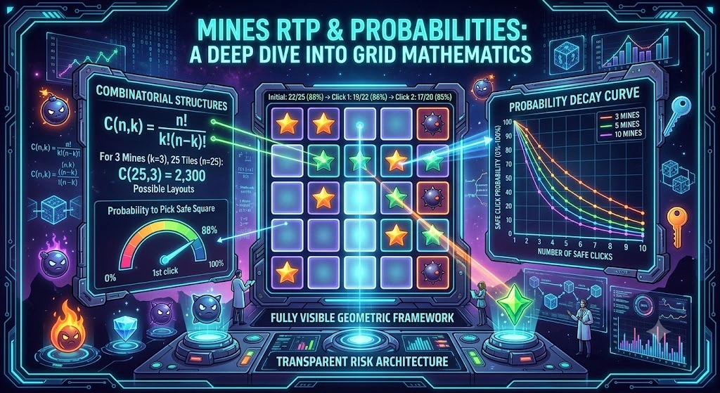
The total universe of possible mine distributions across the board can be determined using the standard combinatorial formula for combinations without repetition:
Let let k represent the number of consecutive safe tiles a player attempts to uncover during a single game loop. The mathematical probability of surviving the very first step (k = 1) is a basic linear ratio of safe tiles to total tiles:
For a standard moderate setup of 5 mines (M = 5), the initial probability of choosing a safe diamond tile is exactly 80%.
However, if that first selection is safe, the entire probability matrix instantly updates for the next choice (k = 2). The total pool of unrevealed tiles drops to 24, and the remaining available safe tiles drop to 19. The conditional probability of surviving the second pick given that the first was successful becomes:
To compute the cumulative probability of surviving a sequence of k consecutive clicks without detonating a mine, we must apply the product of these shifting conditional probabilities:
This equation clearly illustrates the concept of probability decay. With every diamond you pull out of the grid, the relative density of the hidden mines increases within the remaining unclicked tiles, causing your real-time odds of survival to plunge at an accelerating rate.
The Multiplier Equation: How the Payout Scales
To understand how the software enforces its House Edge while allowing you to change the parameters of the game, we must look at how the interface calculates your payout multipliers.
If a casino offered perfectly “fair odds” (a 0% House Edge), your multiplier at any given step $k$ would be the exact mathematical inverse of your cumulative survival probability:
To permanently secure its mathematical advantage, the software provider multiplies this fair payout value by the target RTP coefficient of the game (e.g., 0.99 for a 1% House Edge):
Because the denominator shrinks non-linearly with every successful click, the resulting display multiplier grows along a steep, accelerating curve. The casino does not need to manually manipulate the board mid-game; the raw mathematical decay of your survival odds natively handles the scaling of the payout.
Volatility Mapping: A Comparative Analysis
To see exactly how changing the number of mines shifts the variance landscape without altering the core equity, let us examine a comparative dataset mapped across different user configurations, assuming an industry-standard RTP = 0.99$ (1% House Edge).
Probability and Multiplier Matrix (N=25, RTP=0.99$)
| Configured Mines (M) | Step (k) | Step Success Probability | Cumulative Survival Probability | Actual Display Multiplier |
| 1 Mine | 1 | 24 / 25 = 0.9600 | 0.9600 | 1.03x |
| 2 | 23 / 24 ≈ 0.9583 | 0.9200 | 1.07x | |
| 3 | 22 / 23 ≈ 0.9565 | 0.8800 | 1.12x | |
| 5 Mines | 1 | 20 / 25 = 0.8000 | 0.8000 | 1.23x |
| 2 | 19 / 24 ≈ 0.7916 | 0.6333 | 1.56x | |
| 3 | 18 / 23 ≈ 0.7826 | 0.4956 | 1.99x | |
| 10 Mines | 1 | 15 / 25 = 0.6000 | 0.6000 | 1.65x |
| 2 | 14 / 24 ≈ 0.5833 | 0.3500 | 2.82x | |
| 3 | 13 / 23 ≈ 0.5652 | 0.1978 | 5.00x |
This data mapping perfectly demonstrates the two opposite ends of risk architecture:
The Low-Mine Paradigm (1–2 Mines)
When setting the board to 1 mine, your individual step probability remains incredibly high (>95%) across your opening choices. The cumulative survival probability decays very slowly, resulting in a flat, highly predictable multiplier growth curve. This configuration minimizes short-term session variance, allowing players to build stable, incremental credit grinds. However, the trade-off is extreme asymmetry: a single rare failure requires a prolonged sequence of successful rounds to fully recover your base capital.


The High-Mine Paradigm (15–24 Mines)
When scaling the mine selector to an aggressive level, the mathematical matrix undergoes a massive transformation. If you choose a 24-mine layout, the cumulative survival probability for the very first click drops to a brutal 1 / 25 = 0.04 (4%). Because surviving this event is mathematically rare, the single-click payout instantly spikes to a massive 24.75x your wager. This layout completely bypasses the deep grid journey, condensing the entire volatility profile of a standard slot machine bonus round into a single high-stakes binary interaction.
Conclusion: Mastering the Expected Value Curve
Ultimately, the mathematical mechanics of Mines reveal that no single configuration of the board is inherently “better” or more profitable than another from an equity standpoint. The House Edge remains an immutable, invisible constant locked into the code.
True tactical mastery of the interface relies entirely on aligning your personal capital management with the specific mathematical curve of your chosen setup. By recognizing that changing the mine count merely reformats how your risk is distributed over time, you can remove emotional guesswork, optimize your cash-out targets, and treat the 25-tile grid as the pure exercise in mathematical variance that it truly is.
Mines Mathematical FAQ